Goal of this lecture ¶ Describe the inhomogeneous universe
Perturbation in the metric ∼ 1 0 − 5 \sim 10^{-5} ∼ 1 0 − 5
Anisotropies in photon distribution
Inhomogeneities in matter distribution (linear regime)
Some basis notions ¶ Lights and horizons ¶ The size of a causal patch of space determined how far light can travel in a certain amount of time.
In an expanding spacetime, the propagation of light is studied in conformal time, in the radial direction (θ = ϕ = 0 \theta = \phi = 0 θ = ϕ = 0
d s 2 = a 2 ( τ ) [ d τ 2 − d χ 2 ] ds^2 = a^2(\tau) [d\tau^2 - d\chi^2] d s 2 = a 2 ( τ ) [ d τ 2 − d χ 2 ]
where d χ = d r 1 − k r 2 d\chi = \dfrac{dr}{\sqrt{1 - kr^2}} d χ = 1 − k r 2 d r { k = 1 spherical k = 0 flat k = 1 hyperbolic \begin{cases} k = 1 \quad \text{spherical} \\ k = 0 \quad \text{flat} \\ k = 1 \quad \text{hyperbolic} \end{cases} ⎩ ⎨ ⎧ k = 1 spherical k = 0 flat k = 1 hyperbolic
Photon follows null geodesics d s 2 = 0 ds^2 = 0 d s 2 = 0 45 ° 45\degree 45° χ − τ \chi-\tau χ − τ
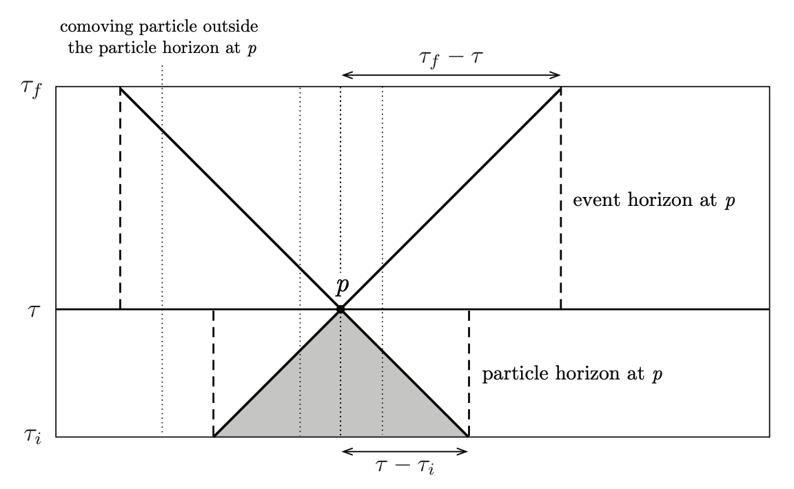
Particle horizon : the maximal comoving distance that light can travel since the Big Bang (τ i ≡ 0 \tau_i \equiv 0 τ i ≡ 0
χ p h ( τ ) = τ − τ i = ∫ t i t d t a ( t ) \chi_{ph}(\tau) = \tau - \tau_i = \int_{t_i}^t \dfrac{dt}{a(t)} χ p h ( τ ) = τ − τ i = ∫ t i t a ( t ) d t This is (comoving) particle horizon .
Event horizon : the maximal comoving distance that light can travel to the future (τ f \tau_f τ f
χ e h ( τ ) = τ f − τ = ∫ t t f d t a ( t ) \chi_{eh}(\tau) = \tau_f - \tau = \int_{t}^{t_f} \dfrac{dt}{a(t)} χ e h ( τ ) = τ f − τ = ∫ t t f a ( t ) d t This is (comoving) event horizon . This can be finite even if the physical time is infinite (τ f = ∞ \tau_f = \infty τ f = ∞
Hubble radius ¶ We can rewrite the particle horizon as
χ p h ( τ ) = ∫ t i t d t a ( t ) = ∫ a i a d a a a ˙ = ∫ ln a i ln a ( a H ) − 1 d ln a \chi_{ph}(\tau) = \int_{t_i}^t \dfrac{dt}{a(t)} = \int_{a_i}^a \dfrac{da}{a \dot a} = \int_{\ln a_i}^{\ln a} (aH)^{-1} d \ln a χ p h ( τ ) = ∫ t i t a ( t ) d t = ∫ a i a a a ˙ d a = ∫ l n a i l n a ( a H ) − 1 d ln a The causal structure of spacetime is related to the comoving Hubble radius
( a H ) − 1 \boxed{(aH)^{-1}
} ( a H ) − 1 For a universe dominated by a fluid with constant equation of state ω = P / ρ \omega = P/\rho ω = P / ρ
( a H ) − 1 = H 0 − 1 a 1 / 2 ( 1 + 3 ω ) , χ p h ( t ) = 2 1 + 3 ω ( a H ) − 1 (aH)^{-1} = H_0^{-1} a^{1/2 (1+3\omega)} \quad, \quad \chi_{ph}(t) = \dfrac{2}{1+3\omega} (aH)^{-1} ( a H ) − 1 = H 0 − 1 a 1/2 ( 1 + 3 ω ) , χ p h ( t ) = 1 + 3 ω 2 ( a H ) − 1 So for normal matters (e.g. baryons, CDM, radiation) with ω > 0 \omega > 0 ω > 0
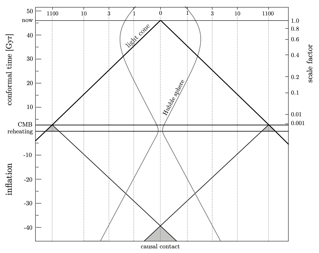
In standard cosmology, the Hubble radius grows as the Universe expands.
Looking backward in time, the particle horizon becomes very small, meaning that widely separated regions of the early Universe were never in causal contact.
However, observations of the Cosmic Microwave Background show that the temperature is homogeneous across the sky at the level
δ T T ∼ 1 0 − 5 , \frac{\delta T}{T} \sim 10^{-5}, T δ T ∼ 1 0 − 5 , which appears inconsistent with this lack of causal connection.
Solution to Horizon Problem ¶ There must be an early phase where the comoving Hubble radius decreases .
This phase is called inflation .
If inflation lasts long enough, regions that we see today were once in causal contact.
d d t ( a H ) − 1 < 0. \frac{d}{dt}(aH)^{-1} < 0 . d t d ( a H ) − 1 < 0. During this time, the Universe expands with acceleration ((\ddot a>0)).
Physical distances grow very fast, faster than the Hubble scale, so a small connected region is stretched to very large scales.
Consequence ¶ We get more conformal time between the Big Bang and photon decoupling.
We need an exotic component with equation of state
w = p ρ < − 1 3 .
w=\frac{p}{\rho}<-\frac{1}{3}. w = ρ p < − 3 1 .
In conformal time, the Big Bang is pushed to very early time
τ i → − ∞ ,
\tau_i \to -\infty, τ i → − ∞ ,
The inhomogeneous universe ¶ Stage 1: Perturbation in the metric ¶ g μ ν = g ˉ μ ν ⏟ FLRW metric + δ g μ ν ⏟ perturbation g_{\mu \nu} = \underbrace{\bar g_{\mu \nu}}_{\text{FLRW metric}} + \underbrace{\delta g_{\mu \nu}}_{\text{perturbation}} g μν = FLRW metric g ˉ μν + perturbation δ g μν The perturbed metric can then be written as
d s 2 = a 2 ( τ ) [ ( 1 + 2 A ) d τ 2 − 2 B i d x i d τ − ( δ i j + h i j ) d x i d x j ] ds^2 = a^2(\tau) \left[ (1+2A) d\tau^2 - 2 B_i dx^i d\tau - (\delta_{ij} + h_{ij}) dx^i dx^j \right] d s 2 = a 2 ( τ ) [ ( 1 + 2 A ) d τ 2 − 2 B i d x i d τ − ( δ ij + h ij ) d x i d x j ] where A A A B i B_i B i h i j h_{ij} h ij
Scalar, Vectors and Tensors ¶ SVT decomposition separates perturbations into scalar, vector, and tensor parts.
At linear order they are independent, so we can study each one separately.
In practice we care mostly about scalar and tensor modes.
Vector modes are not produced in standard inflation and quickly decay as the Universe expands.
They would create a preferred direction, which contradicts the observed homogeneity and isotropy of the early Universe.
For any vector field B \mathbf{B} B R 3 \mathbb{R}^3 R 3
B = ∇ B + B ~ \mathbf{B} = \nabla B + \mathbf{\tilde{B}} B = ∇ B + B ~ where:
∇ B \nabla B ∇ B gradient (curl-free, “longitudinal”)
B ~ \mathbf{\tilde{B}} B ~ divergence-free (∇ ⋅ B ~ = 0 \nabla \cdot \mathbf{\tilde{B}} = 0 ∇ ⋅ B ~ = 0
In Fourier space: B i ( k ) = i k i B ( k ) + B ~ i ( k ) B_i(\mathbf{k}) = i k_i B(\mathbf{k}) + \tilde{B}_i(\mathbf{k}) B i ( k ) = i k i B ( k ) + B ~ i ( k )
i k i B ( k ) i k_i B(\mathbf{k}) i k i B ( k ) k \mathbf{k} k
B ~ i ( k ) \tilde{B}_i(\mathbf{k}) B ~ i ( k ) k ⋅ B ~ ( k ) = 0 \mathbf{k} \cdot \mathbf{\tilde{B}}(\mathbf{k}) = 0 k ⋅ B ~ ( k ) = 0
For a symmetric tensor h i j h_{ij} h ij
The Trace
h a a = 3 C ⇒ C = 1 3 h a a h^a_a = 3C \quad \Rightarrow \quad C = \frac{1}{3}h^a_a h a a = 3 C ⇒ C = 3 1 h a a This is a scalar , the simplest piece.
Remove the Trace
Define the traceless part:
S i j = h i j − C δ i j S_{ij} = h_{ij} - C\delta_{ij} S ij = h ij − C δ ij Now S a a = 0 S^a_a = 0 S a a = 0
Decompose S i j S_{ij} S ij
“What’s the most general traceless symmetric tensor I can build from derivatives of scalar/vector functions?”
Consider all possible derivatives:
From a scalar E E E :
∂ i ∂ j E but this has trace! \partial_i\partial_j E \quad \text{but this has trace!} ∂ i ∂ j E but this has trace! ∇ 2 E = ∂ a ∂ a E \nabla^2 E = \partial^a\partial_a E ∇ 2 E = ∂ a ∂ a E traceless :
∂ i ∂ j E − 1 3 δ i j ∇ 2 E \partial_i\partial_j E - \frac{1}{3}\delta_{ij}\nabla^2 E ∂ i ∂ j E − 3 1 δ ij ∇ 2 E This is pure scalar origin but traceless.
From a vector F i F_i F i :
The symmetric derivative ∂ ( i F j ) = 1 2 ( ∂ i F j + ∂ j F i ) \partial_{(i}F_{j)} = \frac{1}{2}(\partial_i F_j + \partial_j F_i) ∂ ( i F j ) = 2 1 ( ∂ i F j + ∂ j F i )
This also has a trace ∂ a F a \partial^a F_a ∂ a F a
So we must impose ∂ a F a = 0 \partial^a F_a = 0 ∂ a F a = 0
Tensor h ~ i j \tilde{h}_{ij} h ~ ij :
What remains is h ~ i j \tilde{h}_{ij} h ~ ij
Vector decomposition
B i = ∂ i B ⏟ scalar + B i ^ ⏟ vector B_i = \underbrace{\partial_i B}_{\text{scalar}} + \underbrace{\hat{B_i}}_{\text{vector}} B i = scalar ∂ i B + vector B i ^
with ∂ i B i ^ = 0 \partial^i \hat{B_i} = 0 ∂ i B i ^ = 0
Rank-2 tensor decomposition
h i j = 2 C δ i j + 2 ∂ ⟨ i ∂ j ⟩ E + 2 ∂ ( i E ^ j ) + 2 E ^ i j h_{ij} = 2C \delta_{ij} + 2 \partial_{\langle i} \partial_{j \rangle} E + 2 \partial_{( i} \hat{E}_{j )} + 2 \hat{E}_{ij} h ij = 2 C δ ij + 2 ∂ ⟨ i ∂ j ⟩ E + 2 ∂ ( i E ^ j ) + 2 E ^ ij
where
∂ ⟨ i ∂ j ⟩ E ≡ ( ∂ i ∂ j − 1 3 δ i j ∇ 2 ) E ∂ ( i E ^ j ) ≡ 1 2 ( ∂ i E ^ j + ∂ j E ^ i ) \begin{align*}
\partial_{\langle i} \partial_{j\rangle} E & \equiv\left(\partial_i \partial_j-\frac{1}{3} \delta_{i j} \nabla^2\right) E \\
\partial_{(i} \hat{E}_{j)} & \equiv \frac{1}{2}\left(\partial_i \hat{E}_j+\partial_j \hat{E}_i\right)
\end{align*} ∂ ⟨ i ∂ j ⟩ E ∂ ( i E ^ j ) ≡ ( ∂ i ∂ j − 3 1 δ ij ∇ 2 ) E ≡ 2 1 ( ∂ i E ^ j + ∂ j E ^ i )
with ∂ i E i ^ = 0 \partial^i \hat{E_i} = 0 ∂ i E i ^ = 0 ∂ i E i j ^ = 0 \partial^i \hat{E_{ij}} = 0 ∂ i E ij ^ = 0 E i i ^ = 0 \hat{E^i_i} = 0 E i i ^ = 0
The 10 degrees of freedom of the metric is decomposed into
scalars : A , B , C , E → 4 dof vectors : B i ^ , E i ^ → 2 dof tensors : E i j ^ → 2 dof \begin{align*}
&\text{scalars}: A, B, C, E &\to \quad &\text{4 dof} \\
&\text{vectors}: \hat{B_i}, \hat{E_i} &\to \quad &\text{2 dof} \\
&\text{tensors}: \hat{E_{ij}} &\to \quad &\text{2 dof}
\end{align*} scalars : A , B , C , E vectors : B i ^ , E i ^ tensors : E ij ^ → → → 4 dof 2 dof 2 dof Gauge fixing 
Metric perturbations are not uniquely defined because they depend on the choice of coordinates (the gauge).
We choose how to slice spacetime into constant-time hypersurfaces.
We choose spatial coordinates on each slice.
A bad gauge choice can create fictitious perturbations or hide real ones.
⇒ \Rightarrow ⇒ gauge-invariant perturbations , which remain unchanged under a change of coordinates.
Ψ ≡ A + H ( B − E ′ ) + ( B − E ′ ) ′ , Φ ^ i ≡ E ^ i ′ − B ^ i , E ^ i j , Φ ≡ − C − H ( B − E ′ ) + 1 3 ∇ 2 E . \begin{align*}
\Psi & \equiv A+\mathcal{H}\left(B-E^{\prime}\right)+\left(B-E^{\prime}\right)^{\prime}, \quad \hat{\Phi}_i \equiv \hat{E}_i^{\prime}-\hat{B}_i, \quad \hat{E}_{i j}, \\
\Phi & \equiv-C-\mathcal{H}\left(B-E^{\prime}\right)+\frac{1}{3} \nabla^2 E .
\end{align*} Ψ Φ ≡ A + H ( B − E ′ ) + ( B − E ′ ) ′ , Φ ^ i ≡ E ^ i ′ − B ^ i , E ^ ij , ≡ − C − H ( B − E ′ ) + 3 1 ∇ 2 E . To solve the gauge problem, we fix the gauge and keep track of all perturbations (metric and matter).
Newton Gauge ¶ Choose
B = 0 constant-time hypersurfaces orthogonal to worldlines of observers at rest E = 0 induced geometry of the constant-time is isotropic \begin{align*}
B &= 0 \quad \text{\small constant-time hypersurfaces orthogonal to worldlines of observers at rest} \\
E &= 0 \quad \text{\small induced geometry of the constant-time is isotropic}
\end{align*} B E = 0 constant-time hypersurfaces orthogonal to worldlines of observers at rest = 0 induced geometry of the constant-time is isotropic The metric
d s 2 = a 2 ( τ ) [ ( 1 + 2 ψ ) d η 2 − ( 1 − 2 ϕ ) δ i j d x i d x j ] ds^2 = a^2(\tau) [(1 + 2\psi) d\eta^2 - (1-2\phi) \delta_{ij} dx^i dx^j] d s 2 = a 2 ( τ ) [( 1 + 2 ψ ) d η 2 − ( 1 − 2 ϕ ) δ ij d x i d x j ] We just renamed the remaining two metric perturbations,
A ≡ ψ C ≡ − ϕ \begin{align*}
A &\equiv \psi \\
C &\equiv -\phi
\end{align*} A C ≡ ψ ≡ − ϕ Stage 2: Perturbation Einstein equations ¶ Adiabatic fluctuations ¶ Single–field inflation predicts adiabatic initial fluctuations .
This means all perturbations come from the same local shift in time of the background Universe.
At each point ( τ , x ) (\tau, \mathbf{x}) ( τ , x ) τ + δ τ ( x ) \tau + \delta \tau(\mathbf{x}) τ + δ τ ( x )
The local density of species I I I
δ ρ I ( τ , x ) ≡ ρ ˉ I ( τ + δ τ ( x ) ) − ρ ˉ I ( τ ) , . \delta \rho_I(\tau, \mathbf{x}) \equiv \bar{\rho}_I(\tau + \delta \tau(\mathbf{x})) - \bar{\rho}_I(\tau) ,. δ ρ I ( τ , x ) ≡ ρ ˉ I ( τ + δ τ ( x )) − ρ ˉ I ( τ ) , . For small δ τ \delta \tau δ τ
δ ρ I = ρ ˉ I ′ , δ τ ( x ) , . \delta \rho_I = \bar{\rho}_I' , \delta \tau(\mathbf{x}) ,. δ ρ I = ρ ˉ I ′ , δ τ ( x ) , . The key point is that the same δ τ \delta \tau δ τ :
δ τ = δ ρ I ρ ˉ I ′ = δ ρ J ρ ˉ J ′ for all I , J \delta \tau = \frac{\delta \rho_I}{\bar{\rho}_I'} = \frac{\delta \rho_J}{\bar{\rho}_J'} \quad \text{for all } I,J δ τ = ρ ˉ I ′ δ ρ I = ρ ˉ J ′ δ ρ J for all I , J This means all components fluctuate together, with no relative perturbation between species , which defines an adiabatic mode .
Using
ρ I ˉ ′ ∝ ( 1 + ω I ) ρ I \bar{\rho_I}' \propto (1 + \omega_I) \rho_I ρ I ˉ ′ ∝ ( 1 + ω I ) ρ I and define
δ I ≡ δ ρ I ρ I ˉ \delta_I \equiv \dfrac{\delta \rho_I}{\bar{\rho_I}} δ I ≡ ρ I ˉ δ ρ I We have
δ I 1 + ω I = δ J 1 + ω J \dfrac{\delta_I}{1 + \omega_I} = \dfrac{\delta_J}{1 + \omega_J} 1 + ω I δ I = 1 + ω J δ J For matter and radiation components
δ r = 4 3 δ m \delta_r = \dfrac{4}{3} \delta_m δ r = 3 4 δ m Total density perturbation is dominated by background species since δ I \delta_I δ I
δ ρ t o t = ρ ˉ t o t δ t o t = ∑ I ρ I ˉ δ I \rm \delta \rho_{tot} = \bar{\rho}_{tot} \delta_{tot} = \sum_I \bar{\rho_{I}} \delta_I δ ρ tot = ρ ˉ tot δ tot = I ∑ ρ I ˉ δ I Brief on Evolution of fluctuations ¶ Evolution can be related to whether the particles are causally connected to each other.
A standard way to measure whether two particles are causally connected to each other at a given moment is comparing the comoving separation λ \lambda λ comoving Hubble radius ( a H ) − 1 (aH)^{-1} ( a H ) − 1
λ ≫ ( a H ) − 1 → not causally connected → superhorizon λ ≪ ( a H ) − 1 → causally connected → subhorizon \begin{align*}
&\lambda \gg (aH)^{-1} \quad \to \quad &\text{\textbf{not} causally connected} \quad \to \quad &\text{superhorizon} \\
&\lambda \ll (aH)^{-1} \quad \to \quad &\text{causally connected} \quad \to \quad &\text{subhorizon}
\end{align*} λ ≫ ( a H ) − 1 → λ ≪ ( a H ) − 1 → not causally connected → causally connected → superhorizon subhorizon Also, by defining the comoving wave number (scale)
λ = 2 π k ∼ 1 k \lambda = \dfrac{2\pi}{k} \sim \dfrac{1}{k} λ = k 2 π ∼ k 1 We can compare k k k a H aH a H
k ≪ ( a H ) → not causally connected → superhorizon k ≫ ( a H ) → causally connected → subhorizon \begin{align*}
&k \ll (aH) \quad \to \quad &\text{\textbf{not} causally connected} \quad \to \quad &\text{superhorizon} \\
&k \gg (aH) \quad \to \quad &\text{causally connected} \quad \to \quad &\text{subhorizon}
\end{align*} k ≪ ( a H ) → k ≫ ( a H ) → not causally connected → causally connected → superhorizon subhorizon During inflation: Superhorizon modes
For primordial fluctuation
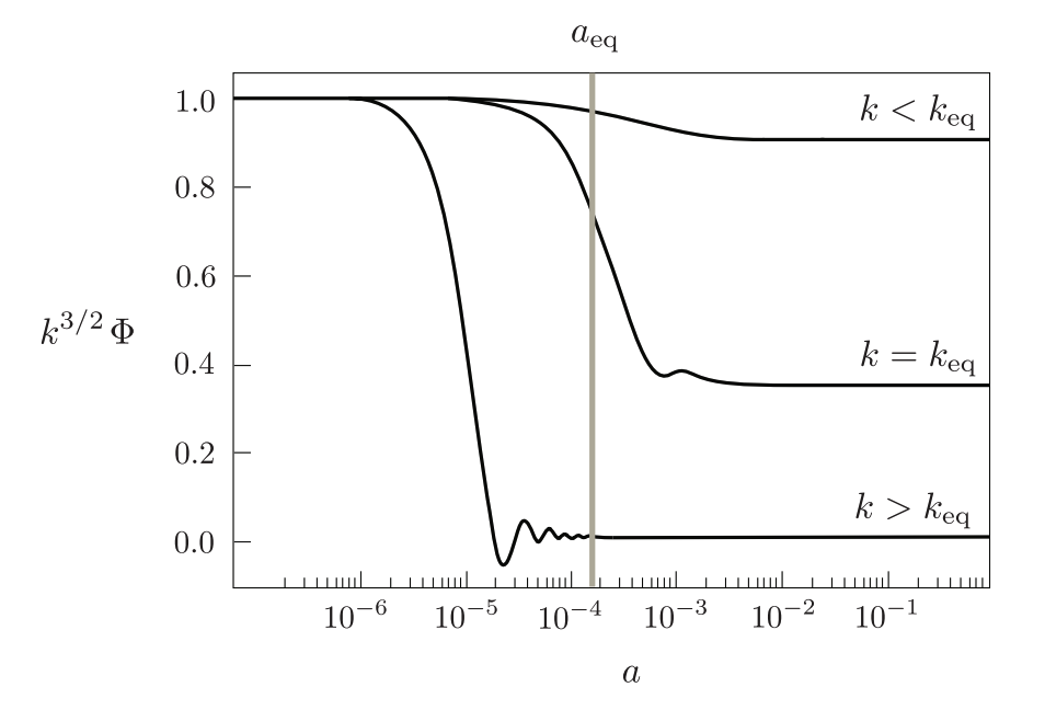
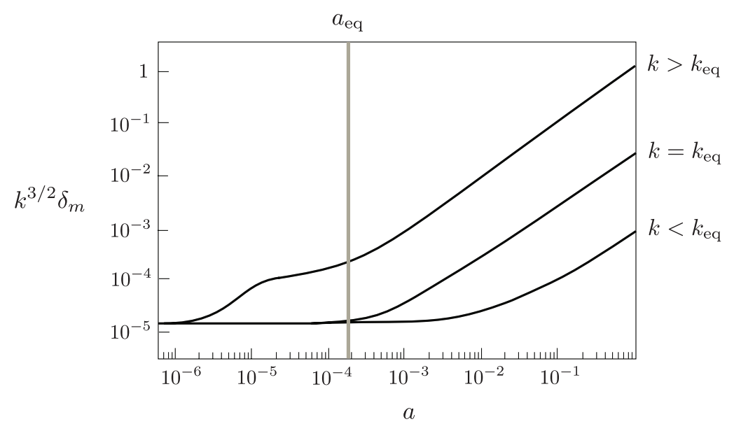
During radiation-dominated era
During matter-dominated era