Skip to article frontmatterSkip to article content
Site not loading correctly?

This may be due to an incorrect BASE_URL configuration. See the MyST Documentation for reference.

Slow-roll inflation

Universite Paris Saclay

Motivation

The Λ\LambdaCDM model is a perfectly satisfactory model of the universe for t103t \gtrsim 10^{-3} s (scales at nuclear reactions), consistent with Big Bang nucleosynthesis, Hubble law, and growth of large-scale structure. However, the initial condition of the model (hot and dense in thermal equilibrium) is not explained.

Therefore, the model is not complete. Λ\LambdaCDM has a number of structure problems/unanswered questions:

These are initial condition problems — and these are what inflation addresses. (What is CDM or what is Λ\Lambda are questions inflation does not address.)

Inflation condition

If we take ρ=constant\rho = \text{constant}, then aeconst×ta \sim e^{\text{const} \times t}, so a¨>0\ddot{a} > 0. But such accelerated expansion never ends, so it cannot be followed by radiation and matter eras. We need a mechanism to realize a finite period of inflation. This leads us to postulate a scalar field.
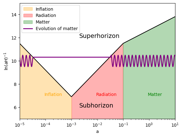
Source:
Inflation
<Figure size 800x400 with 1 Axes>

Figure 1:A schematic for a˙\dot a. We can see that a˙\dot a increases during inflation, then decreases rapidly in the radiation era, decreases more slowly in the matter era, and increases again in the dark energy era.

Are we simply pushing the problem of initial conditions back to tinft_{inf}?

The answer is no, because slow-roll inflation is an attractor solution.

Aspects of inflation

Homogeneous and isotropic cosmology with inflation

Why does inflation solve the flatness and horizon problems? What do you have to do to get a period of primordial inflation? Why is slow roll an attractor solution?

Basic equations

For a Friedmann-Lemaître-Robertson-Walker (FLRW) universe, we have:

{H2=ρ3Mpl2ka2,Mpl2=18πG,k={1closed0flat1opena¨a=4πG3(ρ+3P)ρ˙=3H(ρ+P)\begin{cases} H^2 = \dfrac{\rho}{3 M_{pl}^2} - \dfrac{k}{a^2}, \qquad M_{pl}^2 = \dfrac{1}{8\pi G}, \qquad k = \begin{cases} 1 \quad \text{closed} \\ 0 \quad \text{flat} \\ -1 \quad \text{open} \end{cases} \\[6pt] \dfrac{\ddot{a}}{a} = -\dfrac{4\pi G}{3} (\rho + 3P) \\[6pt] \dot \rho = -3 H (\rho + P) \end{cases}

The comoving Hubble radius

Define the comoving Hubble radius as (aH)1(aH)^{-1}. If atpa \sim t^p, then

(aH)11pt1p.(aH)^{-1} \sim \frac{1}{p} t^{1-p}.

The flatness problem

Define Ω(t)=ρ(t)ρc\Omega(t) = \dfrac{\rho(t)}{\rho_c}, where ρc=3H28πG\rho_c = \dfrac{3 H^2}{8\pi G}. Then

Ω(t)1=Ωk=k(aH)2.\Omega(t) - 1 = \Omega_k = \dfrac{k}{(aH)^2}.

Number of e-folds

Define the number of e-folds as

Nln(aenda).N \equiv \ln\left( \frac{a_{end}}{a} \right).

If a=ainia = a_{ini}, we have

Nln(aendaini).N_\star \equiv \ln\left( \frac{a_{end}}{a_{ini}} \right).

To solve the flatness problem, we need N50N_\star \gtrsim 50.

Quantum fluctuations around the background inflationary solution

How do these become the initial conditions for the Λ\LambdaCDM model?

Source:
Inflation
<Figure size 640x480 with 1 Axes>

Figure 3:Hubble horizon evolution. Scales inside the horizon evolve; scales outside the horizon freeze.

Realizing inflation with a scalar field

Inflation requires a¨>0\ddot{a} > 0, which from the second Friedmann equation implies

ρ+3P<0P<ρ3.\rho + 3P < 0 \quad \Rightarrow \quad P < -\frac{\rho}{3}.

This requires negative pressure. A cosmological constant gives accelerated expansion but never stops. We introduce a scalar field ϕ\phi with a potential V(ϕ)V(\phi) to achieve a finite period of inflation.

If ϕ=const\phi = \text{const}, this is equivalent to a cosmological constant since ρϕ=const\rho_\phi = \text{const}.

Slow-roll inflation: We consider a potential V(ϕ)V(\phi) such that ϕ\phi moves very slowly down the potential.

Scalar field action and equations

The action for a scalar field is

Sϕ=d4xg(12μϕνϕgμνV(ϕ)).S_\phi = \int d^4 x \sqrt{-g} \left( -\frac{1}{2} \partial_\mu \phi \partial_\nu \phi \, g^{\mu \nu} - V(\phi) \right).

The stress-energy tensor is

Tμν=2gδSϕδgμν=μϕνϕgμν(12αϕαϕ+V(ϕ)).T_{\mu \nu} = -\frac{2}{\sqrt{-g}} \frac{\delta S_\phi}{\delta g^{\mu \nu}} = \partial_\mu \phi \partial_\nu \phi - g_{\mu \nu} \left( \frac{1}{2} \partial_\alpha \phi \partial^\alpha \phi + V(\phi) \right).

Varying the action with respect to ϕ\phi gives the Klein-Gordon equation

μμϕ=Vϕ.\nabla_\mu \nabla^\mu \phi = \frac{\partial V}{\partial \phi}.

For a flat FLRW metric gμν=diag(1,a2(t)δij)g_{\mu\nu} = \text{diag}(-1, a^2(t)\delta_{ij}), this becomes

ϕ¨+3Hϕ˙+dVdϕ=0.\boxed{\ddot{\phi} + 3H\dot{\phi} + \frac{dV}{d\phi} = 0}.

From T00T^0_0 and TjiT^i_j, we obtain the energy density and pressure:

ρ=12ϕ˙2+V(ϕ),P=12ϕ˙2V(ϕ).\rho = \frac{1}{2} \dot{\phi}^2 + V(\phi), \qquad P = \frac{1}{2} \dot{\phi}^2 - V(\phi).

Slow-roll conditions

Inflation requires P/ρ1/3P/\rho \ll -1/3, i.e., ϕ˙2V\dot{\phi}^2 \ll V. This is the first slow-roll condition:

Under these conditions, the equations simplify dramatically:

H213Mpl2V(ϕ),3Hϕ˙V(ϕ).H^2 \approx \frac{1}{3M_{pl}^2} V(\phi), \qquad 3H\dot{\phi} \approx -V'(\phi).

Slow-roll parameters

It is convenient to define dimensionless slow-roll parameters in terms of the potential.

Proof 1 (Relation to dynamics)

From the slow-roll equations, we have ϕ˙=V/(3H)\dot{\phi} = -V'/(3H). Substituting into the definition of ϵV\epsilon_V:

ϵV=Mpl22(VV)2=Mpl22(3Hϕ˙V)2.\epsilon_V = \frac{M_{pl}^2}{2} \left( \frac{V'}{V} \right)^2 = \frac{M_{pl}^2}{2} \left( \frac{3H\dot{\phi}}{V} \right)^2.

Using H2V/(3Mpl2)H^2 \approx V/(3M_{pl}^2), we get V3Mpl2H2V \approx 3M_{pl}^2 H^2, so

ϵVMpl22(3Hϕ˙3Mpl2H2)2=12Mpl2(ϕ˙H)2.\epsilon_V \approx \frac{M_{pl}^2}{2} \left( \frac{3H\dot{\phi}}{3M_{pl}^2 H^2} \right)^2 = \frac{1}{2M_{pl}^2} \left( \frac{\dot{\phi}}{H} \right)^2.

This shows ϵV\epsilon_V measures the kinetic energy relative to the potential.

Similarly, one can show that ηV\eta_V measures the acceleration term ϕ¨/(Hϕ˙)\ddot{\phi}/(H\dot{\phi}).

One can also show that

a¨aH2(1ϵV).\frac{\ddot{a}}{a} \approx H^2 (1 - \epsilon_V).

Inflation ends when either ϵV\epsilon_V or ηV|\eta_V| becomes of order 1.

Number of e-folds in terms of the potential

The number of e-folds can be expressed as an integral over the field.

Proof 2 (Number of e-folds)

We have dN=dlna=HdtdN = d\ln a = H dt. Using dt=dϕ/ϕ˙dt = d\phi/\dot{\phi} and the slow-roll relation ϕ˙V/(3H)\dot{\phi} \approx -V'/(3H),

dN=Hdϕϕ˙=H(3HV)dϕ=3H2Vdϕ.dN = H \frac{d\phi}{\dot{\phi}} = H \left( -\frac{3H}{V'} \right) d\phi = -\frac{3H^2}{V'} d\phi.

Using H2V/(3Mpl2)H^2 \approx V/(3M_{pl}^2),

dN=VMpl2Vdϕ.dN = -\frac{V}{M_{pl}^2 V'} d\phi.

Thus the number of e-folds between a field value ϕ\phi and the end of inflation ϕend\phi_{end} is

N(ϕ)=ϕendϕVMpl2Vdϕ.\boxed{N(\phi) = \int_{\phi_{end}}^{\phi} \frac{V}{M_{pl}^2 V'} \, d\phi'}.

Slow-roll inflation is an attractor solution

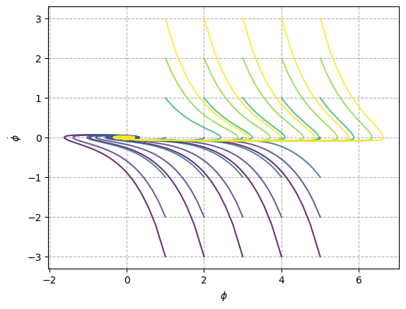
One of the key features of slow-roll inflation is that it is an attractor: independent of the initial conditions (ϕi,ϕ˙i)(\phi_i, \dot{\phi}_i), the solution ϕ(t)\phi(t) converges to the slow-roll trajectory.

We demonstrate this for the quadratic potential V(ϕ)=12m2ϕ2V(\phi) = \frac{1}{2} m^2 \phi^2.

a. The slow-roll solution

From the slow-roll equation 3Hϕ˙=V3H\dot{\phi} = -V', with H2V/(3Mpl2)H^2 \approx V/(3M_{pl}^2):

ϕ˙SR=V3H=m2ϕ3V3Mpl2=m2ϕ3m2ϕ26Mpl2=mMpl3/2ϕϕ.\dot{\phi}_{SR} = -\frac{V'}{3H} = -\frac{m^2 \phi}{3\sqrt{\frac{V}{3M_{pl}^2}}} = -\frac{m^2 \phi}{3\sqrt{\frac{m^2 \phi^2}{6M_{pl}^2}}} = -\frac{m M_{pl}}{\sqrt{3/2}} \frac{\phi}{|\phi|}.

For ϕ>0\phi > 0, ϕ˙SR=23mMpl\dot{\phi}_{SR} = -\sqrt{\frac{2}{3}} m M_{pl} — a constant (negative) velocity.

b. Convergence to the slow-roll solution

We want to show that any trajectory approaches this solution.

dϕ˙dϕ=3Mpl12ϕ˙2+12m2ϕ2m2ϕϕ˙.\frac{d\dot{\phi}}{d\phi} = -\frac{\sqrt{3}}{M_{pl}} \sqrt{\frac{1}{2}\dot{\phi}^2 + \frac{1}{2}m^2\phi^2} - \frac{m^2\phi}{\dot{\phi}}.
Source:
Inflation
<Figure size 640x480 with 1 Axes>

Figure 4:The attractor of inflation: family of phase-space trajectories showing convergence to the slow-roll solution.

Proof 3 (Attractor behavior for quadratic potential)

Start from the full Friedmann and Klein-Gordon equations:

H2=13Mpl2(12ϕ˙2+12m2ϕ2),ϕ¨+3Hϕ˙+m2ϕ=0.H^2 = \frac{1}{3M_{pl}^2} \left( \frac{1}{2} \dot{\phi}^2 + \frac{1}{2} m^2 \phi^2 \right), \qquad \ddot{\phi} + 3H\dot{\phi} + m^2 \phi = 0.

We can study the phase space (ϕ,ϕ˙)(\phi, \dot{\phi}). Define dimensionless variables:

x=ϕMpl,y=ϕ˙mMpl,τ=mt.x = \frac{\phi}{M_{pl}}, \qquad y = \frac{\dot{\phi}}{m M_{pl}}, \qquad \tau = m t.

Then the equations become:

dxdτ=y,dydτ=3H~yx,\frac{dx}{d\tau} = y, \qquad \frac{dy}{d\tau} = -3\tilde{H} y - x,

where H~=H/m=16(y2+x2)\tilde{H} = H/m = \sqrt{\frac{1}{6}(y^2 + x^2)}.

The slow-roll solution corresponds to y=2/3y = -\sqrt{2/3} (for x>0x>0). To study convergence, consider a small deviation: y=2/3+δyy = -\sqrt{2/3} + \delta y, x=xSR+δxx = x_{SR} + \delta x. Linearizing the equations around the slow-roll trajectory shows that perturbations decay exponentially in time, demonstrating that the slow-roll solution is an attractor.

Alternatively, we can derive a first-order equation for ϕ˙(ϕ)\dot{\phi}(\phi). From

dϕ˙dϕ=ϕ¨ϕ˙=3Hϕ˙+m2ϕϕ˙=3Hm2ϕϕ˙.\frac{d\dot{\phi}}{d\phi} = \frac{\ddot{\phi}}{\dot{\phi}} = -\frac{3H\dot{\phi} + m^2\phi}{\dot{\phi}} = -3H - \frac{m^2\phi}{\dot{\phi}}.

Substituting H=13Mpl2(12ϕ˙2+12m2ϕ2)H = \sqrt{\frac{1}{3M_{pl}^2}\left( \frac{1}{2}\dot{\phi}^2 + \frac{1}{2}m^2\phi^2 \right)}, we get

dϕ˙dϕ=3Mpl12ϕ˙2+12m2ϕ2m2ϕϕ˙.\frac{d\dot{\phi}}{d\phi} = -\frac{\sqrt{3}}{M_{pl}} \sqrt{\frac{1}{2}\dot{\phi}^2 + \frac{1}{2}m^2\phi^2} - \frac{m^2\phi}{\dot{\phi}}.

This is a first-order ODE for ϕ˙(ϕ)\dot{\phi}(\phi). The slow-roll solution is a particular solution. One can show numerically (or analytically by linearizing around it) that all trajectories in the phase plane flow toward this solution as ϕ\phi decreases.

Thus, slow-roll inflation is indeed an attractor: regardless of the initial field velocity, the system quickly converges to the slow-roll trajectory, making the predictions of inflation insensitive to initial conditions. This is why inflation solves the fine-tuning problems of the standard Big Bang model.