Linearized GR and Gravitational Waves
Linearized Gravity with Sources and Gravitational Waves ¶ 1. Perturbation theory with sources ¶ We consider a small perturbation around Minkowski spacetime:
g μ ν = η μ ν + h μ ν , ∣ h μ ν ∣ ≪ 1. g_{\mu \nu} = \eta_{\mu \nu} + h_{\mu \nu}, \qquad |h_{\mu \nu}| \ll 1. g μν = η μν + h μν , ∣ h μν ∣ ≪ 1. The linearized Einstein equation in the presence of a stress-energy tensor T μ ν T_{\mu\nu} T μν
G μ ν ( 1 ) ( h α β ) = 8 π G c 4 T μ ν ( 1 ) , G^{(1)}_{\mu \nu}(h_{\alpha \beta}) = \frac{8 \pi G}{c^4} T^{(1)}_{\mu \nu}, G μν ( 1 ) ( h α β ) = c 4 8 π G T μν ( 1 ) , where G μ ν ( 1 ) G^{(1)}_{\mu \nu} G μν ( 1 ) G μ ν ( η α β ) = 0 G_{\mu \nu}(\eta_{\alpha \beta}) = 0 G μν ( η α β ) = 0
1.1 Trace-reversed perturbation ¶ To simplify the left-hand side, we introduce the trace-reversed perturbation:
h ˉ μ ν = h μ ν − 1 2 η μ ν h , h = η μ ν h μ ν , \bar h_{\mu \nu} = h_{\mu \nu} - \frac{1}{2} \eta_{\mu \nu} h, \qquad h = \eta^{\mu \nu} h_{\mu \nu}, h ˉ μν = h μν − 2 1 η μν h , h = η μν h μν , which satisfies h ˉ = − h \bar h = -h h ˉ = − h
1.2 Lorenz gauge condition ¶ We impose the Lorenz gauge condition (also called harmonic gauge):
∂ μ h ˉ μ ν = 0. \partial_\mu \bar h^{\mu \nu} = 0. ∂ μ h ˉ μν = 0. In this gauge, the linearized Einstein equation simplifies dramatically to a wave equation:
□ h ˉ μ ν = − 16 π G c 4 T μ ν , \square \bar h_{\mu \nu} = -\frac{16 \pi G}{c^4} T_{\mu \nu}, □ h ˉ μν = − c 4 16 π G T μν , where □ = η μ ν ∂ μ ∂ ν \square = \eta^{\mu \nu} \partial_\mu \partial_\nu □ = η μν ∂ μ ∂ ν ( 1 ) (1) ( 1 ) T μ ν T_{\mu\nu} T μν
1.3 Conservation of energy-momentum ¶ The stress-energy tensor must satisfy the conservation equation ∇ μ T μ ν = 0 \nabla_\mu T^{\mu \nu} = 0 ∇ μ T μν = 0 h h h Γ T \Gamma T Γ T
∂ μ T μ ν = 0. \partial_\mu T^{\mu \nu} = 0. ∂ μ T μν = 0. At linear order, h h h T μ ν T_{\mu\nu} T μν h μ ν h_{\mu\nu} h μν
2. Gauge freedom and the transverse-traceless gauge ¶ The Lorenz gauge condition (4) x μ → x μ + ϵ μ x^\mu \to x^\mu + \epsilon^\mu x μ → x μ + ϵ μ □ ϵ ν = 0 \square \epsilon^\nu = 0 □ ϵ ν = 0
We can use this freedom to impose two further conditions:
∂ i h ˉ i j = 0 (transverse condition) , \partial^i \bar h_{ij} = 0 \quad \text{(transverse condition)}, ∂ i h ˉ ij = 0 (transverse condition) , h ˉ = 0 (traceless condition) . \bar h = 0 \quad \text{(traceless condition)}. h ˉ = 0 (traceless condition) . From the traceless condition h ˉ = − h = 0 \bar h = -h = 0 h ˉ = − h = 0 h = 0 h = 0 h = 0
h ˉ μ ν = h μ ν . \bar h_{\mu \nu} = h_{\mu \nu}. h ˉ μν = h μν . This combination of conditions (Lorenz + transverse + traceless) defines the transverse-traceless (TT) gauge .
First, solve the wave equation for the spatial components:
□ h ˉ i j = − 16 π G c 4 T i j . \square \bar h_{ij} = -\frac{16 \pi G}{c^4} T_{ij}. □ h ˉ ij = − c 4 16 π G T ij . Then, project the solution onto its transverse-traceless part by imposing h i i = 0 h^i_i = 0 h i i = 0 ∂ i h i j = 0 \partial^i h_{ij} = 0 ∂ i h ij = 0
3. Projection onto TT components ¶ If h ˉ i j \bar h_{ij} h ˉ ij (11) h i j T T h^{TT}_{ij} h ij TT
h i j T T = Λ i j k l ( n ) h ˉ k l , h^{TT}_{ij} = \Lambda_{ij}^{\,\,\, kl}(\mathbf{n}) \, \bar h_{kl}, h ij TT = Λ ij k l ( n ) h ˉ k l , where n \mathbf{n} n
Define the transverse projection operator with respect to a unit vector n \mathbf{n} n
P i j ( n ) = δ i j − n i n j . P_{ij}(\mathbf{n}) = \delta_{ij} - n_i n_j. P ij ( n ) = δ ij − n i n j . Properties:
P i j = P j i P_{ij} = P_{ji} P ij = P ji
P i j n j = 0 P_{ij} n^j = 0 P ij n j = 0 n \mathbf{n} n
P i j P j k = P i k P_{ij} P^{jk} = P_i^{\,k} P ij P jk = P i k
P i j A i = A j T P_{ij}A^i = A^T_j P ij A i = A j T A i = A n i ⏟ longitudinal + A T i ⏟ tranverse A^i = \underbrace{A n^i}_{\text{longitudinal}} + \underbrace{A^{i}_T}_{\text{tranverse}} A i = longitudinal A n i + tranverse A T i
The TT projection operator for a rank-2 tensor is:
Λ i j k l ( n ) = P i k P j l − 1 2 P i j P k l . \Lambda_{ij}^{\,\,\, kl}(\mathbf{n}) = P_i^{\,k} P_j^{\,l} - \frac{1}{2} P_{ij} P^{kl}. Λ ij k l ( n ) = P i k P j l − 2 1 P ij P k l . This operator extracts the transverse, traceless part of a symmetric tensor.
Check that
Λ i j k l δ i j = 0 \Lambda_{ijkl} \delta^{ij} = 0 Λ ijk l δ ij = 0
Λ i j k l n i = 0 \Lambda_{ijkl} n^i = 0 Λ ijk l n i = 0
Λ i k l i = P k i P i l − 1 2 P i i P k l = P k l − P k l = 0 \Lambda^i_{\, \, ikl} = P^i_k P_{il} - \dfrac{1}{2} P^i_i P_{kl} = P_{kl} - P_{kl} = 0 Λ ik l i = P k i P i l − 2 1 P i i P k l = P k l − P k l = 0
P i k P j l n i − 1 2 P i j P k l n i = 0 − 0 = 0 P_{ik} P_{jl} n^i - \dfrac{1}{2} P_{ij} P_{kl} n^i = 0 - 0 = 0 P ik P j l n i − 2 1 P ij P k l n i = 0 − 0 = 0
We have
h i j T T = Λ i j k l ( n ) h ˉ k l = P i k h ˉ k l P l j − 1 2 P i j ( P l k h ˉ k l ) h^{TT}_{ij} = \Lambda_{ij}^{\,\,\, kl}(\mathbf{n}) \, \bar h_{kl} = P_{ik} \bar h^{kl} P_{lj} - \dfrac{1}{2} P_{ij} (P_{lk} \bar h^{kl}) h ij TT = Λ ij k l ( n ) h ˉ k l = P ik h ˉ k l P l j − 2 1 P ij ( P l k h ˉ k l ) h T T = P h P − 1 2 P T r ( P h ) \mathbf{h}^{TT} = \mathbf{P} \mathbf{h} \mathbf{P} - \dfrac{1}{2} \mathbf{P} \rm \, Tr(\mathbf{P} \mathbf{h}) h TT = PhP − 2 1 P Tr ( Ph ) Given a binary system is in ( x , z ) (x, z) ( x , z ) h i j T T h^{TT}_{ij} h ij TT y y y
n = ( 0 1 0 ) ⇒ P i j = ( 1 0 0 0 1 0 0 0 1 ) − ( 0 0 0 0 1 0 0 0 0 ) = ( 1 0 0 0 0 0 0 0 1 ) \mathbf{n} =
\begin{pmatrix}
0 \\ 1 \\ 0
\end{pmatrix} \Rightarrow
P_{ij} = \begin{pmatrix}
1 & 0 & 0 \\
0 & 1 & 0 \\
0 & 0 & 1
\end{pmatrix} -
\begin{pmatrix}
0 & 0 & 0 \\
0 & 1 & 0 \\
0 & 0 & 0
\end{pmatrix} =
\begin{pmatrix}
1 & 0 & 0 \\
0 & 0 & 0 \\
0 & 0 & 1
\end{pmatrix} n = ⎝ ⎛ 0 1 0 ⎠ ⎞ ⇒ P ij = ⎝ ⎛ 1 0 0 0 1 0 0 0 1 ⎠ ⎞ − ⎝ ⎛ 0 0 0 0 1 0 0 0 0 ⎠ ⎞ = ⎝ ⎛ 1 0 0 0 0 0 0 0 1 ⎠ ⎞ P h P = ( 1 0 0 0 0 0 0 0 1 ) ( h 11 h 12 h 13 h 12 h 22 h 23 h 13 h 23 h 33 ) ( 1 0 0 0 0 0 0 0 1 ) = ( h 11 0 h 13 0 0 0 h 13 0 h 33 ) \mathbf{P} \mathbf{h} \mathbf{P} =
\begin{pmatrix}
1 & 0 & 0 \\
0 & 0 & 0 \\
0 & 0 & 1
\end{pmatrix}
\begin{pmatrix}
h_{11} & h_{12} & h_{13} \\
h_{12} & h_{22} & h_{23} \\
h_{13} & h_{23} & h_{33}
\end{pmatrix}
\begin{pmatrix}
1 & 0 & 0 \\
0 & 0 & 0 \\
0 & 0 & 1
\end{pmatrix} =
\begin{pmatrix}
h_{11} & 0 & h_{13} \\
0 & 0 & 0 \\
h_{13} & 0 & h_{33}
\end{pmatrix} PhP = ⎝ ⎛ 1 0 0 0 0 0 0 0 1 ⎠ ⎞ ⎝ ⎛ h 11 h 12 h 13 h 12 h 22 h 23 h 13 h 23 h 33 ⎠ ⎞ ⎝ ⎛ 1 0 0 0 0 0 0 0 1 ⎠ ⎞ = ⎝ ⎛ h 11 0 h 13 0 0 0 h 13 0 h 33 ⎠ ⎞ 1 2 P T r ( P h ) = ( h 11 + h 33 2 0 0 0 0 0 0 0 h 11 + h 33 2 ) \dfrac{1}{2} \mathbf{P} \rm \, Tr(\mathbf{P} \mathbf{h}) =
\begin{pmatrix}
\dfrac{h_{11} + h_{33}}{2} & 0 & 0 \\
0 & 0 & 0 \\
0 & 0 & \dfrac{h_{11} + h_{33}}{2}
\end{pmatrix} 2 1 P Tr ( Ph ) = ⎝ ⎛ 2 h 11 + h 33 0 0 0 0 0 0 0 2 h 11 + h 33 ⎠ ⎞ So
h T T = ( h 11 − h 33 2 0 h 13 0 0 0 h 13 0 − h 11 − h 33 2 ) \mathbf{h}^{TT} = \begin{pmatrix}
\dfrac{h_{11} - h_{33}}{2} & 0 & h_{13} \\
0 & 0 & 0 \\
h_{13} & 0 & -\dfrac{h_{11} - h_{33}}{2}
\end{pmatrix} h TT = ⎝ ⎛ 2 h 11 − h 33 0 h 13 0 0 0 h 13 0 − 2 h 11 − h 33 ⎠ ⎞ This is indeed traceless and tranverse to y \mathbf{y} y
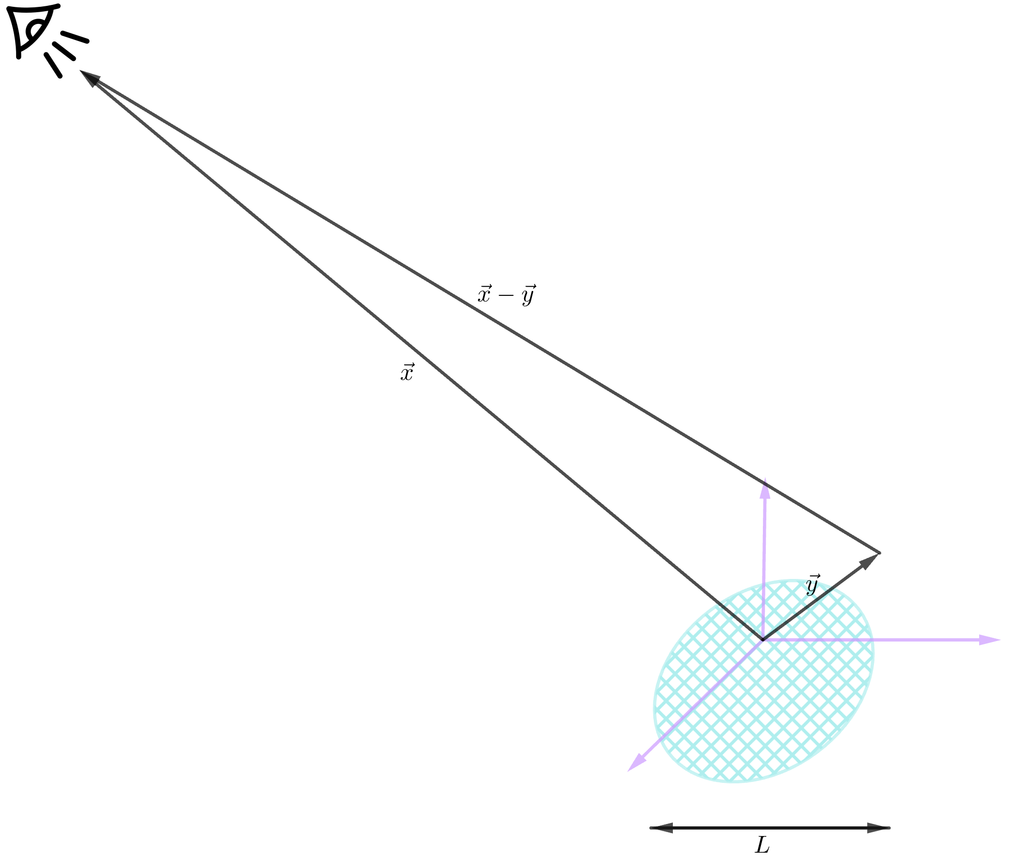
4. Solution of the wave equation with source ¶ Assume the source T i j T_{ij} T ij L L L d d d d ≫ L d \gg L d ≫ L
Figure 1: Geometry for gravitational wave emission: source localized near origin, detector at position x = d n \mathbf{x} = d \mathbf{n} x = d n d ≫ L d \gg L d ≫ L
The solution to (5)
h ˉ i j ( t , x ) = 4 G c 4 ∫ d 3 y 1 ∣ x − y ∣ T i j ( t − ∣ x − y ∣ c , y ) . \bar h_{ij}(t, \mathbf{x}) = \frac{4G}{c^4} \int d^3 y \, \frac{1}{|\mathbf{x} - \mathbf{y}|} \, T_{ij}\left(t - \frac{|\mathbf{x} - \mathbf{y}|}{c}, \mathbf{y}\right). h ˉ ij ( t , x ) = c 4 4 G ∫ d 3 y ∣ x − y ∣ 1 T ij ( t − c ∣ x − y ∣ , y ) . In the far-field limit d ≫ L d \gg L d ≫ L
∣ x − y ∣ ≈ d − n ⋅ y \begin{align*}
|\mathbf{x} - \mathbf{y}| &\approx d - \mathbf{n} \cdot \mathbf{y}
\end{align*} ∣ x − y ∣ ≈ d − n ⋅ y Proof 1 (Expansion of
∣ x − y ∣ |\mathbf{x} - \mathbf{y}| ∣ x − y ∣ )
∣ x − y ∣ = x 2 − 2 x ⋅ y + y 2 = d 1 − 2 x ⋅ y d 2 + y d 2 ⏟ 0 ≈ d ( 1 − 2 x ⋅ y d 2 ) 1 / 2 ≈ d − n ⋅ y \begin{align*}
|\mathbf{x} - \mathbf{y}| &= \sqrt{\mathbb{x}^2 - 2 \mathbf{x} \cdot \mathbf{y} + \mathbf{y}^2} \\
&= d \sqrt{1 - 2 \dfrac{\mathbf{x} \cdot \mathbf{y}}{d^2} + \underbrace{\dfrac{\mathbf{y}}{d^2}}_0} \\
&\approx d \left(1 - 2 \dfrac{\mathbf{x} \cdot \mathbf{y}}{d^2} \right)^{1/2} \\
&\approx d - \mathbf{n} \cdot \mathbf{y}
\end{align*} ∣ x − y ∣ = x 2 − 2 x ⋅ y + y 2 = d 1 − 2 d 2 x ⋅ y + 0 d 2 y ≈ d ( 1 − 2 d 2 x ⋅ y ) 1/2 ≈ d − n ⋅ y giving:
h ˉ i j ( t , x ) ≈ 4 G c 4 d ∫ d 3 y T i j ( t − r c + n ⋅ y c , y ) . \bar h_{ij}(t, \mathbf{x}) \approx \frac{4G}{c^4 d} \int d^3 y \, T_{ij}\left(t - \frac{r}{c} + \frac{\mathbf{n} \cdot \mathbf{y}}{c}, \mathbf{y}\right). h ˉ ij ( t , x ) ≈ c 4 d 4 G ∫ d 3 y T ij ( t − c r + c n ⋅ y , y ) . Expanding in powers of n ⋅ y / c \mathbf{n} \cdot \mathbf{y}/c n ⋅ y / c ∂ μ T μ ν = 0 \partial_\mu T^{\mu\nu}=0 ∂ μ T μν = 0 quadrupole formula :
Proof 2 (Quadrupole formula)
Expansion of T i j T_{ij} T ij
T i j ( t − ∣ x − y ∣ c , y ) = T i j ( t − d c , y ) + y ⋅ n c ∂ t T i j ( t − d c , y ) + ⋯ \begin{align*}
T_{ij} \left( t - \dfrac{|\mathbf{x} - \mathbf{y}|}{c}, \mathbf{y} \right) &= T_{ij} \left( t - \dfrac{d}{c}, \mathbf{y} \right) + \dfrac{\mathbf{y} \cdot \mathbf{n}}{c} \partial_t T_{ij} \left( t - \dfrac{d}{c}, \mathbf{y} \right) + \dotsb
\end{align*} T ij ( t − c ∣ x − y ∣ , y ) = T ij ( t − c d , y ) + c y ⋅ n ∂ t T ij ( t − c d , y ) + ⋯ Characteristic time scale of the source
∂ t T i j ∼ T i j t c \partial_t T_{ij} \sim \dfrac{T_{ij}}{t_c} ∂ t T ij ∼ t c T ij Characteristic velocity
v c = L t c v_c = \dfrac{L}{t_c} v c = t c L Approximation of T i j T_{ij} T ij ∣ y ∣ = L |\mathbf{y}| = L ∣ y ∣ = L
T i j + L c T i j t c + ⋯ = T i j ( 1 + v c c + ⋯ ) T_{ij} + \dfrac{L}{c} \dfrac{T_{ij}}{t_c} + \dotsb = T_{ij}\left(1 + \dfrac{v_c}{c} + \dotsb \right) T ij + c L t c T ij + ⋯ = T ij ( 1 + c v c + ⋯ ) Impose the non-relativistic (slow moving) source v c ≪ c v_c \ll c v c ≪ c
h i j T T ( t , x ) = Λ i j k l 4 G c 4 d ∫ d 3 y T k l ( t − d c , y ) \begin{align*}
h^{TT}_{ij}(t, \mathbf{x}) &= \Lambda_{ij}^{kl} \dfrac{4 G}{c^4 d} \int d^3 \mathbf{y} T_{kl} \left(t - \dfrac{d}{c}, \mathbf{y} \right)
\end{align*} h ij TT ( t , x ) = Λ ij k l c 4 d 4 G ∫ d 3 y T k l ( t − c d , y ) We define
I i j ( t ) = ∫ d 3 y T 00 ( t , y ) y i y j I_{ij}(t) = \int d^3 \mathbf{y} \, T^{00}(t, \mathbf{y}) \, y_i \, y_j I ij ( t ) = ∫ d 3 y T 00 ( t , y ) y i y j
and
S i j = ∫ d 3 y T i j ( t , y ) S_{ij} = \int d^3 \mathbf{y} T_{ij}(t, \mathbf{y}) S ij = ∫ d 3 y T ij ( t , y ) From equation of motion ∂ μ T μ ν \partial_\mu T^{\mu \nu} ∂ μ T μν
{ ∂ 0 T 00 + ∂ k T k 0 = 0 ∂ 0 T 0 j + ∂ k T k j = 0 ⇒ { ∂ 0 T 00 = − ∂ k T k 0 ∂ 0 T 0 j = − ∂ k T k j \begin{cases}
\partial_0 T^{00} + \partial_k T^{k0} &= 0 \\
\partial_0 T^{0j} + \partial_k T^{kj} &= 0
\end{cases} \Rightarrow
\begin{cases}
\partial_0 T^{00} &= - \partial_k T^{k0} \\
\partial_0 T^{0j} &= - \partial_k T^{kj}
\end{cases} { ∂ 0 T 00 + ∂ k T k 0 ∂ 0 T 0 j + ∂ k T kj = 0 = 0 ⇒ { ∂ 0 T 00 ∂ 0 T 0 j = − ∂ k T k 0 = − ∂ k T kj We have
I ˙ i j = ∫ d 3 y ∂ 0 T 00 y i y j = − ∫ d 3 y ∂ k T k 0 y i y j \begin{align*}
\dot I_{ij} &= \int d^3 \mathbf{y} \partial_0 T^{00} \, y_i \, y_j \\
&= - \int d^3 \mathbf{y} \partial_k T^{k0} \, y_i \, y_j
\end{align*} I ˙ ij = ∫ d 3 y ∂ 0 T 00 y i y j = − ∫ d 3 y ∂ k T k 0 y i y j
Integration by part
I ˙ i j = ∫ d 3 y T k 0 [ ( ∂ k y i ) y j + y i ( ∂ k y j ) ] = ∫ d 3 y T k 0 [ δ k i y j + y i δ k j ] = ∫ d 3 y [ T i 0 y j + T j 0 y i ] \begin{align*}
\dot I_{ij} &= \int d^3 \mathbf{y} T^{k0} [(\partial_k y_i) y_j + y_i (\partial_k y_j)] \\
&= \int d^3 \mathbf{y} T^{k0} [\delta_{ki} y_j + y_i \delta_{kj}] \\
&= \int d^3 \mathbf{y} [T_i^0 y_j + T_j^0 y_i]
\end{align*} I ˙ ij = ∫ d 3 y T k 0 [( ∂ k y i ) y j + y i ( ∂ k y j )] = ∫ d 3 y T k 0 [ δ ki y j + y i δ kj ] = ∫ d 3 y [ T i 0 y j + T j 0 y i ] Second derivative
I i j ¨ = ∫ d 3 y [ ( ∂ 0 T i 0 ) y j + ( ∂ 0 T j 0 ) y i ] = − ∫ d 3 y ( ∂ k T k i y j + ∂ k T k j y i ) = 2 S i j ( Integral by part again! ) \begin{align*}
\ddot{I_{ij}} &= \int d^3 \mathbf{y} [(\partial_0 T^{i0}) y_j + (\partial_0 T^{j0})y_i] \\
&= - \int d^3 \mathbf{y} (\partial_k T^{ki} y_j + \partial_k T^{kj} y_i) \\
&= 2 S_{ij} \quad (\text{Integral by part again!})
\end{align*} I ij ¨ = ∫ d 3 y [( ∂ 0 T i 0 ) y j + ( ∂ 0 T j 0 ) y i ] = − ∫ d 3 y ( ∂ k T ki y j + ∂ k T kj y i ) = 2 S ij ( Integral by part again! ) 5. Application to a binary system in circular Kepler orbit ¶ We now apply the linearized theory to the most important source of gravitational waves for ground‑based detectors: a compact binary system (two black holes or neutron stars) in a circular orbit.
5.1 Setup and definitions ¶ Consider two point masses m 1 m_1 m 1 m 2 m_2 m 2 M = m 1 + m 2 M = m_1 + m_2 M = m 1 + m 2 μ = m 1 m 2 M \mu = \dfrac{m_1 m_2}{M} μ = M m 1 m 2
r = y 1 − y 2 , \mathbf{r} = \mathbf{y}_1 - \mathbf{y}_2, r = y 1 − y 2 , and the individual positions are
y 1 = m 2 M r , y 2 = − m 1 M r . \mathbf{y}_1 = \frac{m_2}{M}\mathbf{r},\qquad \mathbf{y}_2 = -\frac{m_1}{M}\mathbf{r}. y 1 = M m 2 r , y 2 = − M m 1 r . For a circular orbit of radius r r r x x x y y y
r ( t ) = r ( cos ( Ω t ) , sin ( Ω t ) , 0 ) , \mathbf{r}(t) = r\bigl(\cos(\Omega t),\; \sin(\Omega t),\; 0\bigr), r ( t ) = r ( cos ( Ω t ) , sin ( Ω t ) , 0 ) , with orbital angular frequency Ω = G M / r 3 \Omega = \sqrt{GM/r^{3}} Ω = GM / r 3
5.2 Quadrupole moment and its second time derivative ¶ The (mass) quadrupole moment is defined by
I i j ( t ) = ∫ d 3 y T 00 ( t , y ) y i y j , I_{ij}(t) = \int d^3y\; T_{00}(t,\mathbf{y})\, y_i y_j, I ij ( t ) = ∫ d 3 y T 00 ( t , y ) y i y j , where for point masses T 00 = ρ T_{00} = \rho T 00 = ρ c = 1 c=1 c = 1
I i j = m 1 y 1 i y 1 j + m 2 y 2 i y 2 j = μ r i r j . I_{ij} = m_1 y_{1i} y_{1j} + m_2 y_{2i} y_{2j}
= \mu \, r_i r_j. I ij = m 1 y 1 i y 1 j + m 2 y 2 i y 2 j = μ r i r j . Thus
I i j ( t ) = 1 2 μ r 2 ( cos ( 2 Ω t ) sin ( 2 Ω t ) 0 sin ( 2 Ω t ) − cos ( 2 Ω t ) 0 0 0 0 ) . I_{ij}(t) = \dfrac{1}{2} \mu\, r^2 \begin{pmatrix}
\cos (2\Omega t) & \sin(2\Omega t) & 0\\
\sin (2\Omega t) & -\cos(2 \Omega t) & 0\\
0 & 0 & 0
\end{pmatrix}. I ij ( t ) = 2 1 μ r 2 ⎝ ⎛ cos ( 2Ω t ) sin ( 2Ω t ) 0 sin ( 2Ω t ) − cos ( 2Ω t ) 0 0 0 0 ⎠ ⎞ . For a circular binary in the x x x y y y
I ¨ i j ( t ) = − 2 μ r 2 Ω 2 ( cos ( 2 Ω t ) sin ( 2 Ω t ) 0 sin ( 2 Ω t ) − cos ( 2 Ω t ) 0 0 0 0 ) . \ddot I_{ij}(t) = -2\mu r^2 \Omega^2
\begin{pmatrix}
\cos(2\Omega t) & \sin(2\Omega t) & 0\\
\sin(2\Omega t) & -\cos(2\Omega t) & 0\\
0 & 0 & 0
\end{pmatrix}. I ¨ ij ( t ) = − 2 μ r 2 Ω 2 ⎝ ⎛ cos ( 2Ω t ) sin ( 2Ω t ) 0 sin ( 2Ω t ) − cos ( 2Ω t ) 0 0 0 0 ⎠ ⎞ . Notice the appearance of 2 Ω 2\Omega 2Ω twice the orbital frequency .
Proof 3 (Derivation of
I ¨ i j \ddot I_{ij} I ¨ ij )
Starting from I i j = μ r i r j I_{ij} = \mu r_i r_j I ij = μ r i r j r = r ( cos Ω t , sin Ω t , 0 ) \mathbf{r} = r(\cos\Omega t,\sin\Omega t,0) r = r ( cos Ω t , sin Ω t , 0 )
I ˙ i j = μ ( r ˙ i r j + r i r ˙ j ) , I ¨ i j = μ ( r ¨ i r j + r i r ¨ j + 2 r ˙ i r ˙ j ) . \begin{aligned}
\dot I_{ij} &= \mu(\dot r_i r_j + r_i \dot r_j),\\
\ddot I_{ij} &= \mu(\ddot r_i r_j + r_i \ddot r_j + 2\dot r_i \dot r_j).
\end{aligned} I ˙ ij I ¨ ij = μ ( r ˙ i r j + r i r ˙ j ) , = μ ( r ¨ i r j + r i r ¨ j + 2 r ˙ i r ˙ j ) . For circular motion,
r = r ( cos θ , sin θ , 0 ) , r ˙ = r Ω ( − sin θ , cos θ , 0 ) , r ¨ = − r Ω 2 ( cos θ , sin θ , 0 ) , \mathbf{r} = r(\cos\theta,\sin\theta,0),\quad
\dot{\mathbf{r}} = r\Omega(-\sin\theta,\cos\theta,0),\quad
\ddot{\mathbf{r}} = -r\Omega^2(\cos\theta,\sin\theta,0), r = r ( cos θ , sin θ , 0 ) , r ˙ = r Ω ( − sin θ , cos θ , 0 ) , r ¨ = − r Ω 2 ( cos θ , sin θ , 0 ) , with θ = Ω t \theta = \Omega t θ = Ω t
For i = j = x i=j=x i = j = x I ¨ x x = μ [ ( − r Ω 2 cos θ ) ( r cos θ ) + ( r cos θ ) ( − r Ω 2 cos θ ) + 2 ( r Ω ( − sin θ ) ) ( r Ω ( − sin θ ) ) ] \ddot I_{xx} = \mu[(-r\Omega^2\cos\theta)(r\cos\theta) + (r\cos\theta)(-r\Omega^2\cos\theta) + 2(r\Omega(-\sin\theta))(r\Omega(-\sin\theta))] I ¨ xx = μ [( − r Ω 2 cos θ ) ( r cos θ ) + ( r cos θ ) ( − r Ω 2 cos θ ) + 2 ( r Ω ( − sin θ )) ( r Ω ( − sin θ ))]
= μ r 2 [ − Ω 2 cos 2 θ − Ω 2 cos 2 θ + 2 Ω 2 sin 2 θ ] = − 2 μ r 2 Ω 2 ( cos 2 θ − sin 2 θ ) = − 2 μ r 2 Ω 2 cos 2 θ . = \mu r^2[-\Omega^2\cos^2\theta -\Omega^2\cos^2\theta + 2\Omega^2\sin^2\theta] = -2\mu r^2\Omega^2(\cos^2\theta - \sin^2\theta) = -2\mu r^2\Omega^2\cos2\theta. = μ r 2 [ − Ω 2 cos 2 θ − Ω 2 cos 2 θ + 2 Ω 2 sin 2 θ ] = − 2 μ r 2 Ω 2 ( cos 2 θ − sin 2 θ ) = − 2 μ r 2 Ω 2 cos 2 θ . For i = j = y i=j=y i = j = y I ¨ y y = − 2 μ r 2 Ω 2 ( sin 2 θ − cos 2 θ ) = + 2 μ r 2 Ω 2 cos 2 θ \ddot I_{yy} = -2\mu r^2\Omega^2(\sin^2\theta - \cos^2\theta) = +2\mu r^2\Omega^2\cos2\theta I ¨ yy = − 2 μ r 2 Ω 2 ( sin 2 θ − cos 2 θ ) = + 2 μ r 2 Ω 2 cos 2 θ
For i = x , j = y i=x,j=y i = x , j = y I ¨ x y = μ [ ( − r Ω 2 cos θ ) ( r sin θ ) + ( r cos θ ) ( − r Ω 2 sin θ ) + 2 ( r Ω ( − sin θ ) ) ( r Ω cos θ ) ] \ddot I_{xy} = \mu[(-r\Omega^2\cos\theta)(r\sin\theta) + (r\cos\theta)(-r\Omega^2\sin\theta) + 2(r\Omega(-\sin\theta))(r\Omega\cos\theta)] I ¨ x y = μ [( − r Ω 2 cos θ ) ( r sin θ ) + ( r cos θ ) ( − r Ω 2 sin θ ) + 2 ( r Ω ( − sin θ )) ( r Ω cos θ )]
= μ r 2 [ − Ω 2 cos θ sin θ − Ω 2 cos θ sin θ − 2 Ω 2 sin θ cos θ ] = − 4 μ r 2 Ω 2 cos θ sin θ = − 2 μ r 2 Ω 2 sin 2 θ . = \mu r^2[-\Omega^2\cos\theta\sin\theta -\Omega^2\cos\theta\sin\theta - 2\Omega^2\sin\theta\cos\theta] = -4\mu r^2\Omega^2\cos\theta\sin\theta = -2\mu r^2\Omega^2\sin2\theta. = μ r 2 [ − Ω 2 cos θ sin θ − Ω 2 cos θ sin θ − 2 Ω 2 sin θ cos θ ] = − 4 μ r 2 Ω 2 cos θ sin θ = − 2 μ r 2 Ω 2 sin 2 θ . The remaining components vanish. This yields the matrix above.
The quadrupole formula (derived in the previous section) gives the transverse‑traceless wave amplitude at a distance d d d n \mathbf{n} n
h i j T T ( t , x ) = 2 G c 4 d Λ i j k l ( n ) I ¨ k l ( t − d c ) . h^{TT}_{ij}(t,\mathbf{x}) = \frac{2G}{c^4 d}\,\Lambda_{ij}^{\,\,\,kl}(\mathbf{n})\, \ddot I_{kl}\!\left(t - \frac{d}{c}\right). h ij TT ( t , x ) = c 4 d 2 G Λ ij k l ( n ) I ¨ k l ( t − c d ) . For a binary observed face‑on (i.e. along the orbital axis), the projection is trivial and the two independent polarisations are simply proportional to the components of I ¨ i j \ddot I_{ij} I ¨ ij
5.3 Wave amplitude and the chirp mass ¶ The non‑zero components of I ¨ i j \ddot I_{ij} I ¨ ij 2 μ r 2 Ω 2 2\mu r^2 \Omega^2 2 μ r 2 Ω 2 h i j h_{ij} h ij
h 0 = 2 G c 4 d ( 2 μ r 2 Ω 2 ) . h_0 = \frac{2G}{c^4 d}\, (2\mu r^2 \Omega^2). h 0 = c 4 d 2 G ( 2 μ r 2 Ω 2 ) . We now eliminate r r r Ω 2 = G M / r 3 \Omega^2 = GM/r^3 Ω 2 = GM / r 3 r r r
r = ( G M Ω 2 ) 1 / 3 . r = \left(\frac{GM}{\Omega^2}\right)^{1/3}. r = ( Ω 2 GM ) 1/3 . Substituting into the amplitude:
h 0 = 4 G μ c 4 d ( G M Ω 2 ) 2 / 3 Ω 2 = 4 G μ c 4 d ( G M ) 2 / 3 Ω 2 − 4 / 3 = 4 G μ c 4 d ( G M ) 2 / 3 Ω 2 / 3 . h_0 = \frac{4G\mu}{c^4 d} \left(\frac{GM}{\Omega^2}\right)^{2/3} \Omega^2
= \frac{4G\mu}{c^4 d} (GM)^{2/3} \Omega^{2 - 4/3}
= \frac{4G\mu}{c^4 d} (GM)^{2/3} \Omega^{2/3}. h 0 = c 4 d 4 G μ ( Ω 2 GM ) 2/3 Ω 2 = c 4 d 4 G μ ( GM ) 2/3 Ω 2 − 4/3 = c 4 d 4 G μ ( GM ) 2/3 Ω 2/3 . It is convenient to introduce the chirp mass , which combines the two masses in a way that simplifies the expression:
M = ( m 1 m 2 ) 3 / 5 ( m 1 + m 2 ) 1 / 5 = μ 3 / 5 M 2 / 5 . \mathcal{M} = \frac{(m_1 m_2)^{3/5}}{(m_1+m_2)^{1/5}} = \mu^{3/5} M^{2/5}. M = ( m 1 + m 2 ) 1/5 ( m 1 m 2 ) 3/5 = μ 3/5 M 2/5 . From this definition, we have μ = M 5 / 3 M − 2 / 3 \mu = \mathcal{M}^{5/3} M^{-2/3} μ = M 5/3 M − 2/3 h 0 h_0 h 0
h 0 = 4 G c 4 d M 5 / 3 M − 2 / 3 ( G M ) 2 / 3 Ω 2 / 3 = 4 G c 4 d M 5 / 3 G 2 / 3 Ω 2 / 3 . h_0 = \frac{4G}{c^4 d} \mathcal{M}^{5/3} M^{-2/3} (GM)^{2/3} \Omega^{2/3}
= \frac{4G}{c^4 d} \mathcal{M}^{5/3} G^{2/3} \Omega^{2/3}. h 0 = c 4 d 4 G M 5/3 M − 2/3 ( GM ) 2/3 Ω 2/3 = c 4 d 4 G M 5/3 G 2/3 Ω 2/3 . Finally, note that the gravitational wave frequency f f f f = Ω / π f = \Omega/\pi f = Ω/ π Ω = π f \Omega = \pi f Ω = π f
The amplitude of gravitational waves from a circular binary, observed at a distance d d d f f f
h 0 = 4 ( G M ) 5 / 3 c 4 d ( π f ) 2 / 3 . \boxed{ h_0 = \frac{4(G\mathcal{M})^{5/3}}{c^4 d} (\pi f)^{2/3} }. h 0 = c 4 d 4 ( G M ) 5/3 ( π f ) 2/3 . Here G M G\mathcal{M} G M ( G M ) 5 / 3 (G\mathcal{M})^{5/3} ( G M ) 5/3
6. Energy carried by gravitational waves ¶ Gravitational waves transport energy and cause the orbit of a binary system to shrink. However, because of the equivalence principle, one cannot define a local stress‑energy tensor for gravity, at any point one can choose a locally inertial frame where the gravitational field (and hence its energy) vanishes. Nevertheless, a meaningful averaged energy‑momentum pseudotensor can be constructed, provided the average is taken over several wavelengths of the radiation.
6.1 The stress‑energy pseudotensor ¶ For a weak gravitational wave h μ ν h_{\mu\nu} h μν Landau–Lifshitz or Isaacson averaged expression:
t μ ν = c 4 32 π G ⟨ ∂ μ h α β ∂ ν h α β ⟩ , t_{\mu\nu} = \frac{c^4}{32\pi G}\, \big\langle \partial_\mu h_{\alpha\beta}\,\partial_\nu h^{\alpha\beta} \big\rangle, t μν = 32 π G c 4 ⟨ ∂ μ h α β ∂ ν h α β ⟩ , where ⟨ ⋯ ⟩ \langle \cdots \rangle ⟨ ⋯ ⟩ z z z t 0 z t^{0z} t 0 z
The pseudotensor is gauge‑dependent, but its average over several wavelengths is gauge‑invariant and physically meaningful.
The factor c 4 / ( 32 π G ) c^4/(32\pi G) c 4 / ( 32 π G )
For a monochromatic wave, one finds that the energy flux F = c t 00 F = c\,t^{00} F = c t 00 c 3 32 π G ω 2 ( h + 2 + h × 2 ) \frac{c^3}{32\pi G}\omega^2 (h_+^2 + h_\times^2) 32 π G c 3 ω 2 ( h + 2 + h × 2 ) h + , h × h_+,\;h_\times h + , h ×
6.2 Energy loss from a binary system ¶ The quadrupole formula derived earlier gives the wave amplitude h i j T T h^{TT}_{ij} h ij TT
P G W = G 5 c 5 ⟨ I ¨ i j I ¨ i j ⟩ , P_{\mathrm{GW}} = \frac{G}{5c^5} \big\langle \ddot I_{ij} \ddot I^{ij} \big\rangle, P GW = 5 c 5 G ⟨ I ¨ ij I ¨ ij ⟩ , where I i j I_{ij} I ij I ¨ i j \ddot I_{ij} I ¨ ij I ¨ i j \ddot I_{ij} I ¨ ij 2 Ω 2\Omega 2Ω
The gravitational wave luminosity of a circular binary is
P G W = 32 5 G 4 c 5 μ 2 M 3 r 5 = 32 5 c 5 G ( G M Ω c 3 ) 10 / 3 . P_{\mathrm{GW}} = \frac{32}{5}\frac{G^4}{c^5} \frac{\mu^2 M^3}{r^5}
= \frac{32}{5}\frac{c^5}{G} \left(\frac{G\mathcal{M}\Omega}{c^3}\right)^{10/3}. P GW = 5 32 c 5 G 4 r 5 μ 2 M 3 = 5 32 G c 5 ( c 3 G M Ω ) 10/3 . Here M = μ 3 / 5 M 2 / 5 \mathcal{M} = \mu^{3/5} M^{2/5} M = μ 3/5 M 2/5 Ω = G M / r 3 \Omega = \sqrt{GM/r^3} Ω = GM / r 3
Proof 4 (Derivation of the power)
Starting from I ¨ i j \ddot I_{ij} I ¨ ij Second time derivative of the quadrupole moment I i j = I i j − 1 3 δ i j I k k I_{ij} = I_{ij} - \frac{1}{3}\delta_{ij} I^k_{\;k} I ij = I ij − 3 1 δ ij I k k x x x y y y I k k = μ r 2 I^k_{\;k} = \mu r^2 I k k = μ r 2
I i j = μ r 2 ( cos 2 Ω t − 1 3 cos Ω t sin Ω t 0 cos Ω t sin Ω t sin 2 Ω t − 1 3 0 0 0 − 1 3 ) . I_{ij} = \mu r^2 \begin{pmatrix}
\cos^2\Omega t - \frac13 & \cos\Omega t\sin\Omega t & 0\\
\cos\Omega t\sin\Omega t & \sin^2\Omega t - \frac13 & 0\\
0 & 0 & -\frac13
\end{pmatrix}. I ij = μ r 2 ⎝ ⎛ cos 2 Ω t − 3 1 cos Ω t sin Ω t 0 cos Ω t sin Ω t sin 2 Ω t − 3 1 0 0 0 − 3 1 ⎠ ⎞ . Differentiating three times and averaging over an orbit (using ⟨ cos 2 2 Ω t ⟩ = ⟨ sin 2 2 Ω t ⟩ = 1 2 \langle \cos^2 2\Omega t\rangle = \langle \sin^2 2\Omega t\rangle = \frac12 ⟨ cos 2 2Ω t ⟩ = ⟨ sin 2 2Ω t ⟩ = 2 1 ⟨ cos 2 Ω t sin 2 Ω t ⟩ = 0 \langle \cos 2\Omega t\sin 2\Omega t\rangle = 0 ⟨ cos 2Ω t sin 2Ω t ⟩ = 0
⟨ I ¨ i j I ¨ i j ⟩ = 32 5 μ 2 r 4 Ω 6 . \big\langle \ddot I_{ij} \ddot I^{ij} \big\rangle = \frac{32}{5} \mu^2 r^4 \Omega^6. ⟨ I ¨ ij I ¨ ij ⟩ = 5 32 μ 2 r 4 Ω 6 . Inserting r 3 = G M / Ω 2 r^3 = GM/\Omega^2 r 3 = GM / Ω 2 μ = M 5 / 3 M − 2 / 3 \mu = \mathcal{M}^{5/3} M^{-2/3} μ = M 5/3 M − 2/3 M \mathcal{M} M Ω \Omega Ω
The total energy of the binary (in the Newtonian approximation) is
E = − G μ M 2 r . E = -\frac{G\mu M}{2r}. E = − 2 r G μ M . As the system loses energy to gravitational waves, r r r
− d E d t = P G W . -\frac{dE}{dt} = P_{\mathrm{GW}}. − d t d E = P GW . Using d E / d r = + G μ M 2 r 2 dE/dr = + \frac{G\mu M}{2r^2} d E / d r = + 2 r 2 G μ M E E E r r r
d r d t = − 64 5 G 3 μ M 2 c 5 r 3 . \frac{dr}{dt} = -\frac{64}{5}\frac{G^3\mu M^2}{c^5 r^3}. d t d r = − 5 64 c 5 r 3 G 3 μ M 2 . Now relate the gravitational wave frequency f = Ω / π f = \Omega/\pi f = Ω/ π r r r f = 1 π G M r 3 f = \frac{1}{\pi}\sqrt{\frac{GM}{r^3}} f = π 1 r 3 GM
d f d t = 3 2 π G M r − 5 / 2 ( − d r d t ) . \frac{df}{dt} = \frac{3}{2\pi}\sqrt{GM}\, r^{-5/2} \left(-\frac{dr}{dt}\right). d t df = 2 π 3 GM r − 5/2 ( − d t d r ) . Substituting d r / d t dr/dt d r / d t f f f M \mathcal{M} M chirp formula :
The rate of change of the gravitational wave frequency for a circular binary is
d f d t = 96 5 π 8 / 3 ( G M c 3 ) 5 / 3 f 11 / 3 . \boxed{ \frac{df}{dt} = \frac{96}{5} \pi^{8/3} \left(\frac{G\mathcal{M}}{c^3}\right)^{5/3} f^{11/3} }. d t df = 5 96 π 8/3 ( c 3 G M ) 5/3 f 11/3 . This equation shows that the frequency increases (“chirps”) on a time scale τ = f / f ˙ ∝ f − 8 / 3 M − 5 / 3 \tau = f/\dot f \propto f^{-8/3} \mathcal{M}^{-5/3} τ = f / f ˙ ∝ f − 8/3 M − 5/3 f f f f ˙ \dot f f ˙ M \mathcal{M} M
Proof 5 (Derivation of the chirp formula)
Start from Kepler’s law: Ω 2 = G M r 3 \Omega^2 = \frac{GM}{r^3} Ω 2 = r 3 GM Ω = π f \Omega = \pi f Ω = π f
r = ( G M ( π f ) 2 ) 1 / 3 . r = \left(\frac{GM}{(\pi f)^2}\right)^{1/3}. r = ( ( π f ) 2 GM ) 1/3 . The binary energy is E = − G μ M 2 r = − G μ M 2 ( ( π f ) 2 G M ) 1 / 3 E = -\frac{G\mu M}{2r} = -\frac{G\mu M}{2} \left(\frac{(\pi f)^2}{GM}\right)^{1/3} E = − 2 r G μ M = − 2 G μ M ( GM ( π f ) 2 ) 1/3
d E d t = − G μ M 2 ⋅ 1 3 ( ( π f ) 2 G M ) − 2 / 3 ⋅ 2 π 2 f d f d t ⋅ 1 G M = − π 2 3 μ ( G M ( π f ) 2 ) 2 / 3 f d f d t . \frac{dE}{dt} = -\frac{G\mu M}{2} \cdot \frac{1}{3} \left(\frac{(\pi f)^2}{GM}\right)^{-2/3} \cdot 2\pi^2 f \frac{df}{dt} \cdot \frac{1}{GM}
= -\frac{\pi^2}{3} \mu \left(\frac{GM}{(\pi f)^2}\right)^{2/3} f \frac{df}{dt}. d t d E = − 2 G μ M ⋅ 3 1 ( GM ( π f ) 2 ) − 2/3 ⋅ 2 π 2 f d t df ⋅ GM 1 = − 3 π 2 μ ( ( π f ) 2 GM ) 2/3 f d t df . Now use the relation between μ \mu μ M M M μ = M 5 / 3 M − 2 / 3 \mu = \mathcal{M}^{5/3} M^{-2/3} μ = M 5/3 M − 2/3 ( G M / ( π f ) 2 ) 2 / 3 = ( G M ) 2 / 3 ( π f ) − 4 / 3 (GM/(\pi f)^2)^{2/3} = (GM)^{2/3} (\pi f)^{-4/3} ( GM / ( π f ) 2 ) 2/3 = ( GM ) 2/3 ( π f ) − 4/3
d E d t = − π 2 3 M 5 / 3 M − 2 / 3 ( G M ) 2 / 3 ( π f ) − 4 / 3 f d f d t = − π 2 − 4 / 3 3 M 5 / 3 G 2 / 3 f 1 − 4 / 3 d f d t = − 1 3 π 2 / 3 ( G M ) 5 / 3 f − 1 / 3 d f d t . \frac{dE}{dt} = -\frac{\pi^2}{3} \mathcal{M}^{5/3} M^{-2/3} (GM)^{2/3} (\pi f)^{-4/3} f \frac{df}{dt}
= -\frac{\pi^{2-4/3}}{3} \mathcal{M}^{5/3} G^{2/3} f^{1-4/3} \frac{df}{dt}
= -\frac{1}{3} \pi^{2/3} (G\mathcal{M})^{5/3} f^{-1/3} \frac{df}{dt}. d t d E = − 3 π 2 M 5/3 M − 2/3 ( GM ) 2/3 ( π f ) − 4/3 f d t df = − 3 π 2 − 4/3 M 5/3 G 2/3 f 1 − 4/3 d t df = − 3 1 π 2/3 ( G M ) 5/3 f − 1/3 d t df . Set this equal to the GW luminosity from Eq. Gravitational wave luminosity of a circular binary
P G W = 32 5 c 5 G ( G M Ω c 3 ) 10 / 3 = 32 5 c 5 G ( G M ) 10 / 3 ( π f ) 10 / 3 c − 10 = 32 5 ( G M ) 10 / 3 ( π f ) 10 / 3 1 G c 5 . P_{\mathrm{GW}} = \frac{32}{5} \frac{c^5}{G} \left(\frac{G\mathcal{M}\Omega}{c^3}\right)^{10/3}
= \frac{32}{5} \frac{c^5}{G} (G\mathcal{M})^{10/3} (\pi f)^{10/3} c^{-10}
= \frac{32}{5} (G\mathcal{M})^{10/3} (\pi f)^{10/3} \frac{1}{G c^5}. P GW = 5 32 G c 5 ( c 3 G M Ω ) 10/3 = 5 32 G c 5 ( G M ) 10/3 ( π f ) 10/3 c − 10 = 5 32 ( G M ) 10/3 ( π f ) 10/3 G c 5 1 . Equating − d E / d t = P G W -dE/dt = P_{\mathrm{GW}} − d E / d t = P GW E E E
1 3 π 2 / 3 ( G M ) 5 / 3 f − 1 / 3 d f d t = 32 5 ( G M ) 10 / 3 ( π f ) 10 / 3 1 G c 5 . \frac{1}{3} \pi^{2/3} (G\mathcal{M})^{5/3} f^{-1/3} \frac{df}{dt}
= \frac{32}{5} (G\mathcal{M})^{10/3} (\pi f)^{10/3} \frac{1}{G c^5}. 3 1 π 2/3 ( G M ) 5/3 f − 1/3 d t df = 5 32 ( G M ) 10/3 ( π f ) 10/3 G c 5 1 . Cancel a factor ( G M ) 5 / 3 (G\mathcal{M})^{5/3} ( G M ) 5/3 d f / d t df/dt df / d t
d f d t = 3 ⋅ 32 5 ( G M ) 5 / 3 π 10 / 3 − 2 / 3 f 10 / 3 + 1 / 3 1 G c 5 = 96 5 π 8 / 3 ( G M c 3 ) 5 / 3 f 11 / 3 . \frac{df}{dt} = 3 \cdot \frac{32}{5} (G\mathcal{M})^{5/3} \pi^{10/3 - 2/3} f^{10/3 + 1/3} \frac{1}{G c^5}
= \frac{96}{5} \pi^{8/3} \left(\frac{G\mathcal{M}}{c^3}\right)^{5/3} f^{11/3}. d t df = 3 ⋅ 5 32 ( G M ) 5/3 π 10/3 − 2/3 f 10/3 + 1/3 G c 5 1 = 5 96 π 8/3 ( c 3 G M ) 5/3 f 11/3 . All factors of G G G c c c G M / c 3 G\mathcal{M}/c^3 G M / c 3
The chirp formula is the basis for matched‑filtering searches in gravitational wave data analysis. By fitting the observed f ( t ) f(t) f ( t ) M \mathcal{M} M
The derivation assumes the orbit remains circular and that the radiation reaction is slow (adiabatic approximation), which is excellent during the inspiral phase.